library(GeoMagR)
library(GeoPressureR)
library(maps)
library(withr)
library(ggplot2)
tag <- with_dir(system.file("extdata", package = "GeoMagR"), {
tag_create("14DM", quiet = TRUE) |>
tag_label(quiet = TRUE)
})
tagThis vignette walks through the GeoMagR workflow on the bundled Bee-eater tag 14DM. We first inspect the raw sensor data, then calibrate the magnetic measurements with geomag_calib(), and finally build a magnetic likelihood map with geomag_map().
1. Load the sample tag
We start by loading the sample data bundled with the package. GeoMagR builds on top of GeoPressureR, so we use the standard pipeline to create and label a GeoPressureR tag object with tag_create() and tag_label().
tag_label() uses the labeled acceleration data to identify flight periods and create stationary periods (stap).
We can check the orientation of the sensor:
tag$param$mag_axis
#> [1] "left" "backward" "down"The raw magnetic measurements are:
| date | magnetic_x | magnetic_y | magnetic_z | acceleration_x | acceleration_y | acceleration_z | stap_id |
|---|---|---|---|---|---|---|---|
| 2015-07-15 00:00:00 | 0.30368 | 0.12848 | -0.14048 | -1.0158691 | 0.1159058 | 0.2175903 | 1 |
| 2015-07-15 04:00:00 | -0.02016 | -0.26800 | -0.37840 | -0.4349365 | -0.0131836 | 1.9647217 | 1 |
| 2015-07-15 08:00:00 | -0.19648 | 0.05904 | -0.42176 | -0.3776245 | -0.1152954 | 1.1094971 | 1 |
| 2015-07-15 12:00:00 | 0.09968 | 0.16864 | -0.33072 | -0.9479370 | -0.1127319 | 0.7674561 | 1 |
| 2015-07-15 16:00:00 | 0.28208 | -0.12928 | -0.22688 | -0.9280396 | -0.0083618 | 1.0251465 | 1 |
| 2015-07-15 20:00:00 | 0.26384 | -0.12560 | -0.26272 | -1.0314331 | -0.0047607 | 0.1928101 | 1 |
2. Inspect the raw acceleration
Confusingly, the SOI sensor stores activity and mean_acceleration_z as tag$acceleration, while the true 3-axis acceleration data is stored in tag$magnetic. Typically, activity is sampled every 5-30 minutes, while 3-axis acceleration-magnetic data is sampled at a coarser 4-6 hour interval. In this vignette, and in GeoMagR in general, we use the 3-axis acceleration.
We can visualize acceleration in a 3D scatter plot. We add a unit sphere to show the value at rest (only gravity acts on the sensor). With our left-backward-down reference frame, gravity should have a positive z axis when the logger is perfectly horizontal, but the logger on the bird’s back is typically slightly tilted backward (negative x axis). Here, our bee-eater spends a significant part of its time with its back fully vertical (x ~ -1 g, z ~ 0 g).
plot_mag(
tag,
type = "acceleration",
static_thr_hard = 0.1,
static_thr_outlier = 3
)3. Inspect the raw magnetic field
The next plot shows the three magnetic axes in sensor coordinates.
Each color indicates a different stationary period, where the bird is assumed to stay at the same location. Points with the same color lie on the same radius of the sphere, indicating that the magnetic intensity/magnitude is the same. As the bird moves south, the field intensity decreases, resulting in the points moving closer to the center. At the same time, near the equator, the magnetic field becomes more horizontal, resulting in a point lying on a ring closer to the center of the sphere.
plot_mag(tag, type = "magnetic")We can see that the sphere is not exactly centered at (0, 0, 0): our next step is to correct that offset with magnetic calibration.
4. Calibrate the magnetic sensor
With geomag_calib(), we compute the main magnetic quantities of interest: intensity F, inclination I, and heading H. The function performs tilt compensation and magnetic calibration, with additional pre- and post-processing steps documented in the help page.
For 14DM, we do not have laboratory calibration data, so we use field-data calibration with calib_method = "ellipse_stap" because stationary period information is available.
tag <- geomag_calib(
tag,
calib_data = FALSE, # use field-data calibration
calib_method = "ellipse_stap",
rm_outlier = TRUE
)We can now plot the magnetic data again. This time the fitted calibration ellipsoid is shown. By default, the smallest and largest radii are displayed. The fitted parameters are stored in tag$param$geomag_calib.
plot_mag(tag, type = "magnetic")The tag$magnetic table is now enriched with several calibrated variables. See the geomag_calib() documentation for the full list.
| date | magnetic_x | magnetic_y | magnetic_z | acceleration_x | acceleration_y | acceleration_z | stap_id | is_static | magnetic_xc | magnetic_yc | magnetic_zc | pitch | roll | acceleration_xp | acceleration_yp | acceleration_zp | magnetic_xcp | magnetic_ycp | magnetic_zcp | F | I | H |
|---|---|---|---|---|---|---|---|---|---|---|---|---|---|---|---|---|---|---|---|---|---|---|
| 2015-07-15 00:00:00 | 0.30368 | 0.12848 | -0.14048 | -1.0158691 | 0.1159058 | 0.2175903 | 1 | TRUE | 0.4067842 | 0.1464498 | -0.1333816 | 1.3327149 | 0.4894476 | 0 | 0 | 1.045356 | 0.0484440 | 0.1919634 | -0.4068352 | 0.4524507 | 1.1178948 | 104.163482 |
| 2015-07-15 04:00:00 | -0.02016 | -0.26800 | -0.37840 | -0.4349365 | -0.0131836 | 1.9647217 | 1 | FALSE | 0.0925555 | -0.2544572 | -0.3765927 | 0.2178549 | -0.0067101 | 0 | 0 | 2.012331 | 0.0093435 | -0.2569784 | -0.3860205 | 0.4638286 | 0.9831503 | 267.917692 |
| 2015-07-15 08:00:00 | -0.19648 | 0.05904 | -0.42176 | -0.3776245 | -0.1152954 | 1.1094971 | 1 | FALSE | -0.0756131 | 0.0754742 | -0.4236223 | 0.3264234 | -0.1035452 | 0 | 0 | 1.177657 | -0.2092319 | 0.0312842 | -0.3822471 | 0.4368862 | 1.0653019 | 8.503838 |
| 2015-07-15 12:00:00 | 0.09968 | 0.16864 | -0.33072 | -0.9479370 | -0.1127319 | 0.7674561 | 1 | FALSE | 0.2101541 | 0.1871661 | -0.3298224 | 0.8849994 | -0.1458474 | 0 | 0 | 1.224860 | -0.1405072 | 0.1372456 | -0.3865231 | 0.4335651 | 1.1006444 | 44.327229 |
| 2015-07-15 16:00:00 | 0.28208 | -0.12928 | -0.22688 | -0.9280396 | -0.0083618 | 1.0251465 | 1 | FALSE | 0.3844867 | -0.1136632 | -0.2207560 | 0.7357053 | -0.0081565 | 0 | 0 | 1.382842 | 0.1375176 | -0.1154600 | -0.4209994 | 0.4576927 | 1.1676465 | 220.016872 |
| 2015-07-15 20:00:00 | 0.26384 | -0.12560 | -0.26272 | -1.0314331 | -0.0047607 | 0.1928101 | 1 | TRUE | 0.3668531 | -0.1098205 | -0.2576843 | 1.3859400 | -0.0246863 | 0 | 0 | 1.049311 | -0.1831227 | -0.1161477 | -0.4074540 | 0.4615657 | 1.0817148 | 327.614619 |
First, the calibrated magnetic data tag$magnetic_*c. The measurements are now centered on the origin and lie on a regular sphere, with a radius that still varies slightly by stationary period.
plot_mag(tag, type = "magnetic_c")The reprojected corrected magnetic data tag$magnetic_*cp shows the magnetic field in the horizontal plane of the Earth frame after tilt compensation. The ellipsoid rings are now horizontal, correcting for the bird position.
plot_mag(tag, type = "magnetic_cp")Finally, we can also plot the magnetic values as a time series, showing the raw data and the mean value per stationary period.
plot_mag(tag, type = "timeseries")5. Compute the magnetic likelihood map
Once the tag has been calibrated and the map extent has been defined, geomag_map() can compare the observed field against the World Magnetic Model.
First, we define the spatio-temporal parameters of the map with tag_set_map().
tag <- tag_set_map(
tag,
extent = c(-18, 23, 0, 50),
scale = 2,
known = data.frame(
stap_id = c(1, -1),
known_lon = 7.27,
known_lat = 46.19
)
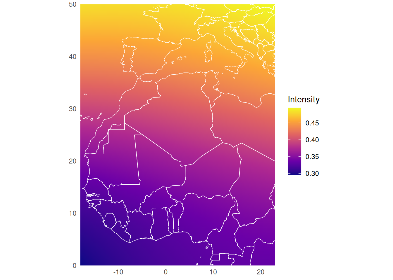
)This reference map is normally computed automatically inside geomag_map(), but we show it explicitly here for clarity.
ref_map = geomag_map_ref(tag)
ref_map_df <- terra::as.data.frame(ref_map$intensity, xy = TRUE)
names(ref_map_df)[3] <- "intensity"
world <- map_data("world")
ggplot(ref_map_df, aes(x = x, y = y, fill = intensity)) +
geom_raster(interpolate = TRUE) +
geom_path(
data = world,
aes(long, lat, group = group),
color = "white",
linewidth = 0.25,
inherit.aes = FALSE
) +
coord_quickmap(xlim = c(-18, 23), ylim = c(0, 50), expand = FALSE) +
scale_fill_viridis_c(option = "C", name = "Intensity") +
labs(x = NULL, y = NULL) +
theme_minimal(base_size = 11) +
theme(
panel.grid = element_blank(),
legend.position = "right"
)
The likelihood computation requires four standard deviations that control the expected measurement error and uncertainty.
For an observation (y_j) and the WMM value (x_s) at candidate location (s), GeoMagR uses
[ y_j = x_s + b + e_j, e_j (0, _e^2), b (0, _m^2). ]
The observation error (_e) describes variation among individual measurements, while the stationary-period error (_m) describes uncertainty shared by all observations from that period. Intensity values and errors are in Gauss; inclination values and errors are in degrees.
tag <- geomag_map(
tag,
compute_known = FALSE,
sd_e_f = 0.009,
sd_e_i = 2.6,
sd_m_f = 0.014,
sd_m_i = 3.5,
ref_map = ref_map
)The defaults provide a practical starting point, but results should be checked with a sensitivity analysis. Increasing either standard deviation broadens the likelihood surface and reduces the influence of magnetic data. Compare trajectories across plausible lower and upper values, especially when calibration quality or logger orientation is uncertain.
The result is a spatial likelihood surface for each stationary period.
plot(tag, "map_magnetic_intensity")We can also add a water mask, here just as an example for inclination.
if (requireNamespace("rnaturalearth", quietly = TRUE)) {
tag$map_magnetic_inclination <- map_add_mask_water(
tag$map_magnetic_inclination
)
}
plot(tag, "map_magnetic_inclination")6. What this workflow gives you
At this point, the tag object contains calibrated magnetic data, a magnetic likelihood map, and all the metadata needed to continue into a GeoPressureR workflow.
The same pattern can be adapted to a real deployment by replacing the bundled sample tag with your own GeoPressureR tag object and changing the map extent to match the study region.