Movement Model with Magnetic Likelihoods

This vignette shows how to run a GeoPressureR movement graph model using magnetic likelihoods from GeoMagR.

It uses the same bundled Bee-eater tag as the first vignette (14DM) and follows the same logic as the Trajectory chapter of the GeoPressureManual:

prepare a tagged object,
compute likelihood maps,
create the graph,
define the movement model,
extract trajectory products.

The difference is that we explicitly include magnetic likelihoods in the graph model.

1. Load and prepare the sample tag (`14DM`)

As in the manual, we start by preparing all required components on the tag object:

tag data (tag_create() and tag_label()),
twilight information for the light map,
map settings (extent, resolution, and known sites).

library(GeoMagR)
library(GeoPressureR)
library(withr)

tag <- with_dir(system.file("extdata", package = "GeoMagR"), {
  tag_create("14DM", quiet = TRUE) |>
    tag_label(quiet = TRUE) |>
    twilight_create() |>
    twilight_label_read() |>
    tag_set_map(
      extent = c(-18, 23, 0, 50),
      scale = 2,
      known = data.frame(
        stap_id = c(1, -1),
        known_lon = 7.27,
        known_lat = 46.19
      )
    )
})

This gives a complete input object for the three observation models used below.

2. Compute likelihood maps

The graph model combines observation likelihoods across sensors. Here we compute magnetic, light, and pressure maps in sequence.

We start with magnetic calibration and magnetic likelihood maps:

tag <- geomag_calib(tag)
tag <- geomag_map(tag)

Then we compute the light and pressure likelihood maps:

tag <- geolight_map(tag, quiet = TRUE)

tag <- geopressure_map(tag, quiet = TRUE)

3. Create the graph

As described in the manual, graph_create() keeps likely nodes and compatible transitions between consecutive stationary periods. The likelihood argument defines which maps are multiplied in the observation model.

graph <- graph_create(
  tag,
  likelihood = c("map_pressure", "map_light", "map_magnetic"),
  thr_likelihood = 0.95,
  thr_gs = 100,
  quiet = TRUE
)

thr_likelihood controls how many candidate nodes are retained at each stationary period, while thr_gs limits transitions to realistic ground speed.

4. Define the movement model

We then convert speed to transition probability with a gamma movement model. This mirrors the default trajectory workflow in the GeoPressureManual.

graph <- graph_set_movement(
  graph,
  method = "gamma",
  shape = 7,
  scale = 7,
  zero_speed_ratio = 15
)
plot_graph_movement(graph)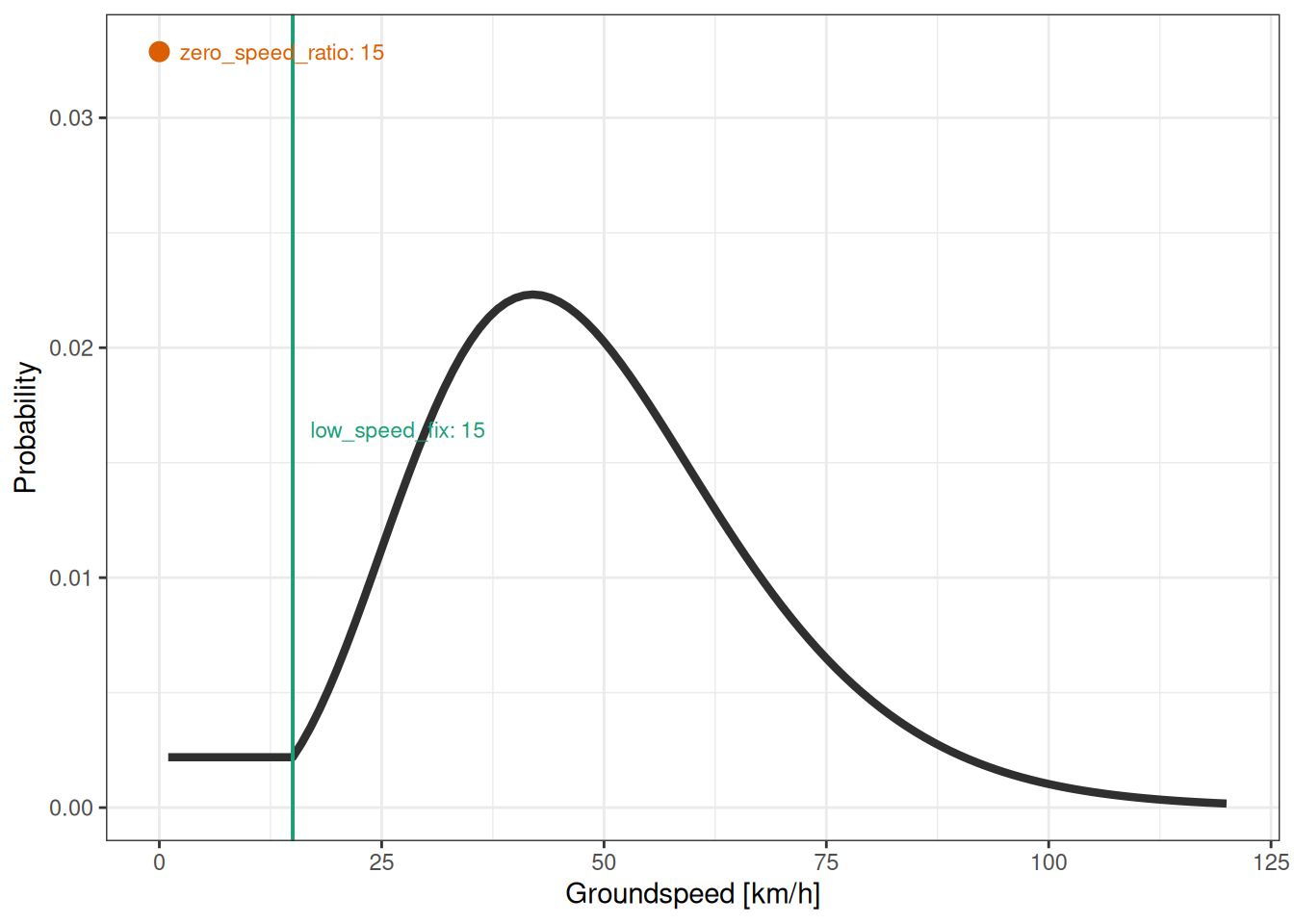

5. Compute trajectory products

We compute the most likely path (Viterbi) and the marginal probability map (forward-backward), following the same product logic as in the manual.

path_most_likely <- graph_most_likely(graph, quiet = TRUE)

marginal <- graph_marginal(graph, quiet = TRUE)

plot(marginal, path = path_most_likely)

6. Practical notes

For a full project workflow (including saved interim outputs and batch processing), see GeoPressureTemplate workflow.

As emphasized in the manual, always inspect: