
Show setup code
library(GeoPathSampleR)
library(GeoPressureR)
knitr::opts_knit$set(
root.dir = system.file("extdata", package = "GeoPathSampleR")
)This vignette uses a light-only example tag bundled with GeoPathSampleR. It shows the complete workflow from raw geolocator data to sampled paths. The example is intentionally short and uses coarse settings so that it can be run while learning the workflow; it is not intended as a scientific analysis.
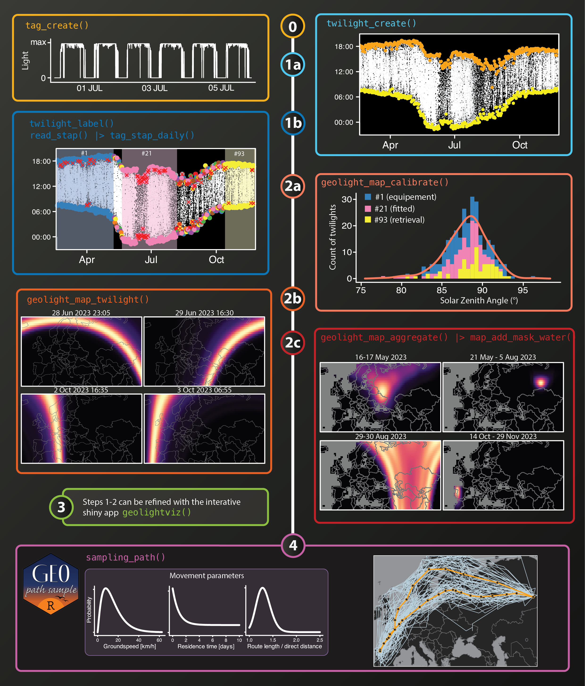
Figure 1 shows the two parts of the workflow. Part I uses GeoPressureR to turn curated twilights into stationary-period likelihood maps, with GeoLightViz supporting interactive review. Part II uses GeoPathSampleR to combine those maps with movement priors and sample posterior trajectories. The sections below follow this order; the Light map chapter of the GeoPressureManual documents Part I in more detail.
library(GeoPathSampleR)
library(GeoPressureR)
knitr::opts_knit$set(
root.dir = system.file("extdata", package = "GeoPathSampleR")
)We recommend using GeoPressureTemplate as the starting point for your analysis. It provides a folder structure where all files for the analysis have their standardized location. Check the instruction on the dedicated GeoPressureManual chapter.
Here, we use the 14OI example contained in the GeoPathSampleR package. The vignette working directory is set to the package’s extdata folder, so GeoPressureR can use its standard relative paths.
Create a tag reads the sensor files from data/raw-tag/{id}. The 14OI example contains light data only, so assert_pressure = FALSE is required. Use crop_start and crop_end to define the period of the data when on the bird.
tag <- tag_create(
"14OI",
crop_start = "2015-07-17",
crop_end = "2016-07-11",
assert_pressure = FALSE,
quiet = TRUE
)Estimating twilights converts the light time series into sunrise and sunset observations.
tag <- twilight_create(tag)Labelling twilights is done interactively with geolightviz.
geolightviz(tag)Once you have exported the label file to data/twilight-label/{id}-labeled.csv, read those labels with:
tag <- twilight_label_read(tag)
plot(tag, type = "twilight")Standard GeoPressureR workflows use acceleration and pressure data to identify flight and stationary periods. This light-only example cannot use those signals, so long stationary periods are identified visually from the twilight plot instead.
Define long stationary periods (stap0) manually with geolightviz and save them in data/stap-label/{id}.csv.
geolightviz(tag)Unlike a standard GeoPressureR analysis, we create daily stationary periods during migration. tag_stap_daily() starts with the long stationary periods (stap0) and fills the gaps with daily periods, grouping twilights according to whether movement is assumed to occur during the night or the day.
tag <- tag_stap_daily(
tag,
stap_long = tag$param$id,
movement_period = "day",
quiet = TRUE
)Revising long periods
After
tag_stap_daily(),tag$stapcontains the daily periods as well as the long periods. To revise the long periods in GeoLightViz, start again withtag_create(),twilight_create(), andtwilight_label_read()before openinggeolightviz(tag). Save the reviseddata/stap-label/{id}.csv, then reruntag_stap_daily()and the following steps.
Defining a map sets the spatial extent and grid resolution used by the likelihood maps. This step comes after stationary periods have been defined because the map uses them as its temporal dimension. The example does not contain known coordinates, so calibration is fitted automatically from the long stationary periods.
tag <- tag |>
tag_set_map(
extent = c(-20, 40, -11, 60),
scale = 1
)Warning
For this example, we assume that no known location is available. This should be rare in a real study, but it illustrates calibration from fitted locations. When known deployment or recovery coordinates are available, include them in
tag_set_map(known = ...)instead.
This is a good place to check the twilight labels and the long and daily stationary periods with geolightviz. You can re-export the labels as needed and rerun the previous steps. The likelihood map is computed in the next section.
geolightviz(tag)Constructing light likelihoods uses the twilight observations and map definition to estimate a light likelihood for each stationary period.
tag <- geolight_map(
tag,
twl_calib_adjust = 1,
fitted_location_duration = 30,
twl_llp = \(n) 1.5 * log(n) / n,
quiet = TRUE
)Note
The arguments used here differ from the GeoPressureR defaults and follow the calibration described in the GeoTwilight analysis (see the relevant appendix):
fitted_location_duration = 30uses long stationary periods, including the non-breeding location, as fitted calibration periods.twl_calib_adjust = 1is used instead of1.4because the fitted calibration periods represent a broader range of twilight errors. The influence is small, and values between 1 and 1.4 are reasonable alternatives.twl_llp = \(n) 1.5 * log(n) / napplies the calibrated pooling weight for workflows combining long and daily stationary periods. Do not transfer this value automatically to workflows with multiple stationary-period durations defined from acceleration data.
The calibration describes the distribution of twilight errors, expressed as solar zenith angles, used to build every likelihood map. Inspect it before continuing: the histogram shows the zenith angles of the calibration twilights, coloured by calibration period (here all fitted from long periods), and the black curve shows the fitted distribution used by the likelihood. A calibration period whose histogram departs strongly from the others can indicate mislabelled twilights or a period that is not stationary.
plot_twl_calib(tag)For landbird, a water mask removes cells from the set of locations that can be sampled.
tag$map_light <- map_add_mask_water(tag$map_light)
plot(tag, type = "map_light")Warning in default_backend_auto(): Selecting 'env' backend. Secrets are stored
in environment variables
Warning in default_backend_auto(): Selecting 'env' backend. Secrets are stored
in environment variables
Warning in default_backend_auto(): Selecting 'env' backend. Secrets are stored
in environment variablesThe movement model implemented in sampling_path() combines three sources of information to define the trajectory:
The movement model defines the daily transition between consecutive stationary periods. It has two parts:
method, shape, scale, low_speed_fix, zero_speed_ratio), evaluated with GeoPressureR::speed2prob(). Speed is the displacement between two consecutive periods divided by 24 h. The default is a Gamma distribution with shape 1.26 and scale 10.3 km/h.move_stay(t), where t is the number of consecutive days already spent at the current location. The default declines exponentially from p_0 = 0.607 just after arrival to a plateau p_inf = 0.137 with time constant tau = 0.932 days. move_stay_parameters only stores these values for plot_movement(); the sampler uses move_stay.The default movement argument of sampling_path() is sampling_path_default_movement(), calibrated on multi-sensor tracks of land birds. We write it out below to show its structure; movement <- sampling_path_default_movement() gives the same list. See ?sampling_path_default_movement for details.
movement <- list(
method = "gamma",
shape = 1.26,
scale = 10.3,
low_speed_fix = 0.001,
zero_speed_ratio = 0,
move_stay_parameters = list(
p_0 = 0.607,
p_inf = 0.137,
tau = 0.932
),
move_stay = function(t) 0.137 + (0.607 - 0.137) * exp(-t / 0.932)
)
plot_movement(movement)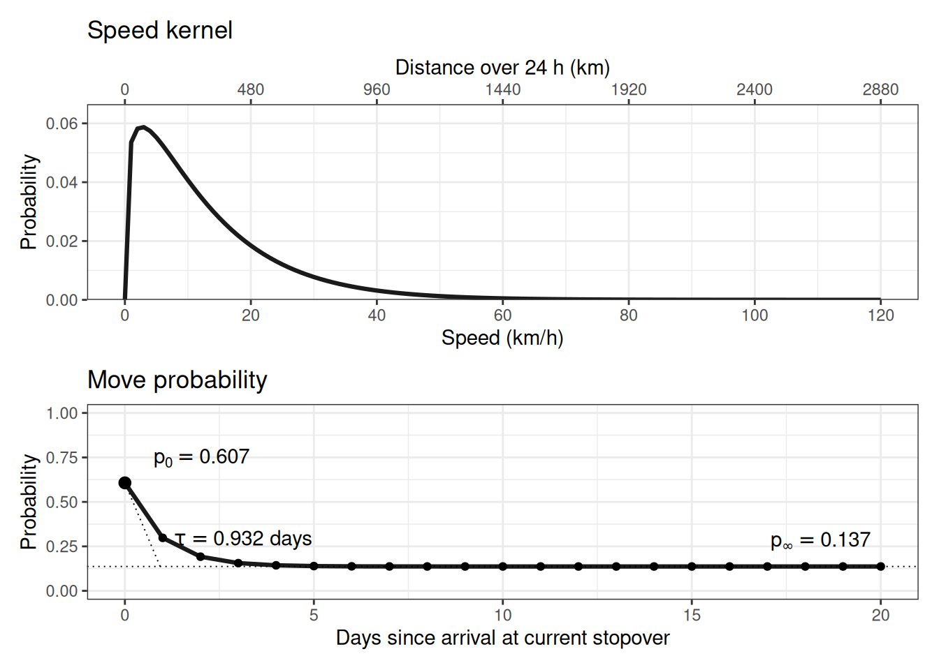
The other arguments of sampling_path() that change the scientific model are:
component_weights = c(light = 1, movement = 1, route = 1) uses each component without rescaling. Each weight scales that component’s log probability, so changing even all three weights by the same factor changes the sampled distribution. Setting a weight to zero removes that component’s soft contribution while retaining hard support constraints; use this only for an explicit sensitivity analysis.route_detour = 1 keeps the calibrated route prior. The value multiplies the expected excess route distance (route length over direct distance, minus one) between consecutive long periods. For instance, for a prior mean route is 19% longer than direct; 2 doubles this excess, 0.5 halves it and 0 favours direct routes.long_period_light_only = TRUE applies a modular cut: unknown long-period locations are drawn from their light likelihood alone, and movement only informs the daily periods between them. FALSE lets movement also update long periods.The following arguments control computation and diagnostics rather than the scientific model:
| Argument | Default | Role and practical choice |
|---|---|---|
iter |
none | Total iterations per chain, including warmup. Increase it when effective sample sizes are too small. |
warmup |
floor(iter / 4) |
Initial iterations discarded while the chain reaches its typical posterior region. |
thin |
1 |
Saving interval. The number saved is floor((iter - warmup) / thin). Keep 1 unless storage is limiting; thinning does not improve mixing. |
chains |
1 |
Number of independent chains. Use at least four for final inference. |
block_interval |
2 |
Frequency of block updates, which move a whole stay at once. Keep the optimized default unless explicitly comparing sampler efficiency. |
thr_likelihood |
0.99 |
Retained light-likelihood mass used to reduce the state space. The conservative default is appropriate for final inference. |
thr_gs |
2000 / 24 |
Hard truncation of the speed kernel, in km/h (2000 km per day). Speeds are already weighted by the movement model, so set it above the speeds the kernel supports rather than at typical speeds; the default excludes less than 0.1% of the default kernel. Larger values cost computation; smaller values forbid transitions outright. |
workers |
1 |
Number of parallel workers for independent chains. Use 1 while debugging and increase only when appropriate for the system. |
seed |
NULL |
Random-number seed for reproducible chains. |
The sampler uses Gibbs updates: it repeatedly updates one stationary-period location, or a block of locations, conditional on the current values of the other periods. The resulting draws are correlated, so the run must be long enough to explore the posterior and must be checked with multiple independent chains.
Begin with a short run to verify that the likelihood, movement support, and route prior are compatible. This run is for checking the workflow, not for inference.
paths <- sampling_path(
tag,
movement = movement,
iter = 500,
chains = 4,
warmup = 100,
seed = 1,
quiet = TRUE
)Inspect convergence and computational-support diagnostics before interpreting a trajectory. The interactive report provides an overview of sampled paths, traces, R-hat, effective sample sizes, chain separation, and warnings about likelihood or movement boundaries.
For interactive review, generate the report with:
diagnostic <- sampling_path_diagnostic(paths, tag, report = TRUE)An example of the resulting report is available on the diagnostic example page.
Once the first run shows no problem with the likelihood, movement support or route prior, run longer chains for inference. Increase iter and warmup until R-hat is close to one and effective sample sizes are large enough for the quantities of interest, and check the diagnostics again before interpreting the paths. The settings below are illustrative only; a real analysis usually needs more iterations.
paths <- sampling_path(
tag,
movement = movement,
iter = 1000,
chains = 4,
warmup = 500,
seed = 1,
quiet = TRUE
)
sampling_path_diagnostic(paths, tag, report = FALSE)paths contains one row per posterior draw and stationary period: each draw is a complete trajectory, and daily periods spent at the same location appear as repeated rows. Two functions turn it into something easier to interpret, and they answer different questions:
path_collapse() works within each draw. It merges consecutive periods assigned to the same grid cell into a single stay, so each draw becomes a sequence of stays and moves. All draws are kept, and so is the posterior uncertainty.path_summary() works across draws. It reduces the ensemble to a single path, either one position per stationary period (by = "stap") or one position per consensus stay (by = "consensus_stay").| Summary | Call | One row per | Keeps uncertainty |
|---|---|---|---|
| Collapsed draws | path_collapse(paths, tag$stap) |
stay of each draw | yes |
| Mean path | path_summary(paths, tag$stap, by = "stap") |
stationary period | no |
| Consensus path | path_summary(paths, tag$stap, by = "consensus_stay") |
consensus stay | no |
We draw ten posterior trajectories at random and collapse each into its stays.
set.seed(1)
path_ids <- unique(paths[c("chain", "j")])
path_ids <- path_ids[sample.int(nrow(path_ids), 10), ]
draws <- merge(paths, path_ids) |>
path_collapse(tag$stap)With by = "stap", path_summary() summarises the positions of all draws separately for each stationary period, here with the mean. With by = "consensus_stay", it first estimates the probability of a move at each boundary between consecutive periods as the proportion of draws whose location changes there. Boundaries with a probability above move_threshold = 0.5 define the consensus stays, and positions are then summarised over all draws and periods of each stay. The columns move_probability_start and move_probability_end report how clear each boundary is.
mean_path <- path_summary(paths, tag$stap, by = "stap", position = "mean")
consensus <- path_summary(paths, tag$stap, by = "consensus_stay")
head(consensus[c("stap_id_start", "stap_id_end", "lat", "lon", "move_probability_end")]) stap_id_start stap_id_end lat lon move_probability_end
1 1 1 52.73375 12.194375 0.92125
2 2 2 50.23687 9.748750 0.69125
3 3 6 47.89875 7.747656 0.53625
4 7 7 46.71000 6.577500 0.78375
5 8 22 42.96771 3.972083 0.88500
6 23 23 35.80000 6.774375 0.93500Figure 2 overlays the three summaries.
draws$j <- interaction(draws$chain, draws$j, drop = TRUE)
mean_path$j <- 1
consensus$j <- 1
map_extent <- tag$param$tag_set_map$extent
map <- leaflet::leaflet(
height = 700,
options = leaflet::leafletOptions(zoomControl = TRUE)
) |>
leaflet::addProviderTiles("Esri.WorldTopoMap") |>
leaflet::fitBounds(
lng1 = map_extent[1],
lat1 = map_extent[3],
lng2 = map_extent[2],
lat2 = map_extent[4]
)
map <- GeoPressureR::plot_path(
draws,
map = map,
group = "Posterior draws",
polyline = list(color = "#8C8C8C", weight = 2, opacity = 0.45),
circle = list(radius = 1, stroke = FALSE, fillOpacity = 0)
)
map <- GeoPressureR::plot_path(
mean_path,
map = map,
group = "Posterior mean",
polyline = list(
color = "#2E8B57",
weight = 4,
opacity = 1,
dashArray = "8, 6"
),
circle = list(radius = 1, stroke = FALSE, fillOpacity = 0)
)
GeoPressureR::plot_path(
consensus,
map = map,
group = "Consensus",
polyline = list(color = "#C26D22", weight = 5, opacity = 1),
circle = list(radius = 1, stroke = FALSE, fillOpacity = 0)
) |>
leaflet::addLayersControl(
overlayGroups = c("Posterior draws", "Posterior mean", "Consensus"),
options = leaflet::layersControlOptions(collapsed = TRUE)
)The three summaries should not be interpreted as interchangeable estimates: