16 Compare studies with the Master

A single GeoLocator Data Package describes one study (see Reuse a study). The Master GeoLocator Data Package compiles every published package of the geolocator-dp Zenodo community into one standardised dataset, released once a year with its own DOI. It is the starting point for questions that no single study can answer.

The first part of this chapter shows how to read the Master, choose source packages and select birds. The second part uses it to describe how songbirds and other small migrants stop, fly, and use the wind, across all tracked species.

library(GeoLocatoR)
library(tidyverse)
options(knitr.kable.NA = "")

Plot theme

theme_set(
  theme_minimal(base_size = 12) +
    theme(
      panel.grid.minor = element_blank(),
      plot.title.position = "plot",
      plot.title = element_text(face = "bold"),
      legend.position = "bottom",
      legend.text = element_text(size = 8),
      legend.key.size = unit(0.4, "cm")
    )
)

16.1 Get started

16.1.1 Read and save a release

Each release has a version DOI, the one to read and cite, and all releases share a concept DOI (10.5281/zenodo.18187092) that always resolves to the latest one. The download is about 1 GB, mostly the in-flight pressurepaths.

master <- read_zenodo("18187093")

Download it once and write it to disk with write_gldp(). Later sessions read the local copy with read_gldp(), which is much faster and works offline:

write_gldp(master, "data/master_2026.0")
master <- read_gldp("data/master_2026.0")

The Master has the same tables as any GeoLocator DP, but no measurements: it holds trajectories, not raw sensor data. It adds a catalogue of its source packages in master$datapackages, with one row per package.

16.1.2 Choose the source packages

The catalogue describes each package: its access status, species, number of tracked birds, sensors and their sampling intervals, and whether its trajectories were computed with wind. It lists every package of the community, including embargoed ones, whose data will join the public tables once their embargo ends.

catalogue <- master$datapackages |>
  mutate(
    project = str_remove(title, "^Geo[Ll]ocator Data Package: "),
    pressure_min = map_dbl(str_split(samplingInterval_pressure_min, "; "), \(x) max(as.numeric(x)))
  )

Code

catalogue |>
  arrange(access_status, desc(numberTags_paths)) |>
  select(project, access_status, numberTags_paths, pressure_min, trajectories_with_wind_pct) |>
  knitr::kable(col.names = c("Project", "Access", "Trajectories", "Pressure interval (min)", "With wind (%)"))

Project	Access	Trajectories	Pressure interval (min)	With wind (%)
Geolocator tracking study of Common Starlings in Latvia	embargoed	40	30	100
UK Pied Flycatcher	embargoed	13	30	100
Common Chiffchaff and Iberian Chiffchaff in Spain	embargoed	12	20	100
Eurasian Wrynecks from Germany	embargoed	9	5	100
European Rollers (Coracias garrulus) in Hungary, Romania and Montenegro	embargoed	8	30	100
Marsh Wabler from Luxembourg	embargoed	6	20	100
Thrush Nightingales from Czechia	embargoed	6	5	100
Spotted Ground Thrush from Durban, ZA	embargoed	4	5	100
Common Starling from Denmark	embargoed	1	5	100
Scops Owl (MIGRALIGHT)	embargoed		5
Kirtland’s Warblers from Michigan, USA	embargoed		20
Painted Buntings from Oklahoma, South Carolina, Georgia, USA	embargoed		20
Alpine swifts	embargoed		30
MIGRATLANE - Monitoring and studying birds in the North-East Atlantic Arc	open	49	20	0
Great Reed Warbler tracks from three European populations	open	32	30	100
Swiss Hoopoes	open	21	30	100
Red-capped Robin-Chat and Mangrove Kingfisher from Kenya	open	18	10	100
Trajectories of Northern Wheatears breeding in Val Piora (Switzerland) and Val Troncea (Italy)	open	13	30	0
Swainson’s Warbler Migration Ecology	open	13	30	100
Thursh nightingale Luscinia Luscinia in South Sweden	open	11	60	0
Red-backed Shrike in Denmark	open	10	60	0
Tawny Pipits from Czechia	open	7	30	100
Eurasian Hoopoes from Germany	open	7	5	100
Myrtle Warbler (Anchorage, AK)	open	6	20	0
Siberian Rubythroat from China	open	6	60	100
South African Woodland Kingfisher	open	5	30	100
Migration Route of Swiss Ring Ouzels	open	5	5	100
Snow Bunting from Svalbard	open	4	60	100
Eurasian Nightjar from Mongolia	open	3	5	100
Western Black-eared Wheatear migration	open	3	60	100
Barred Warblers from Czechia	open	2	30	100
Lesser Grey Shrike in Slovakia	open	1	30	100
White-chested Alethe from Tanzania	open		20

Filter the catalogue like any tibble. For a study of flight behaviour, you may want open packages with high-resolution pressure and trajectories computed with wind:

selected <- catalogue |>
  filter(access_status == "open", pressure_min <= 5, trajectories_with_wind_pct == 100)

Other useful filters include the time span (temporal_start, temporal_end), the sensors (numberTags_light, numberTags_activity, …), or the authors (str_detect(contributors, "Hahn")).

Each tag knows its source package through tags()$datapackage_id. select_gldp() then keeps the rows of the chosen tags in every table:

hires <- tags(master) |>
  filter(datapackage_id %in% selected$datapackage_id) |>
  pull(tag_id) |>
  select_gldp(pkg = master)

This keeps 15 trajectories from 3 packages.

16.1.3 Select birds by what they did

The selection can come from any table. For instance, all birds that spent more than a month in the Sahel, the semi-arid belt south of the Sahara:

sahel <- staps(master) |>
  filter(as.numeric(difftime(end, start, units = "days")) > 30) |>
  inner_join(filter(paths(master), type == "most_likely"), by = c("tag_id", "stap_id")) |>
  filter(between(lat, 10, 18), between(lon, -18, 40)) |>
  distinct(tag_id) |>
  pull(tag_id) |>
  select_gldp(pkg = master)

master$species holds the AviList taxonomy of every species of the Master, which gives English names and a taxonomic order:

species <- bind_rows(master$species) |>
  select(scientific_name = scientific_name_input, species = English_name_AviList, Sequence)

Code

paths(sahel) |>
  filter(type == "most_likely") |>
  left_join(tags(sahel), by = "tag_id") |>
  left_join(species, by = "scientific_name") |>
  mutate(species = fct_infreq(species)) |>
  ggplot(aes(lon, lat)) +
  annotation_borders("world", fill = "grey95", colour = "grey75", linewidth = 0.2) +
  annotate("rect", xmin = -18, xmax = 40, ymin = 10, ymax = 18, fill = NA, colour = "black", linetype = "dashed") +
  geom_path(aes(group = tag_id, colour = species), alpha = 0.5, linewidth = 0.4) +
  scale_colour_manual(values = hcl.colors(15, "Dark 3"), guide = guide_legend(ncol = 3, override.aes = list(alpha = 1, linewidth = 1))) +
  coord_quickmap(xlim = c(-20, 45), ylim = c(-30, 62)) +
  labs(x = NULL, y = NULL, colour = NULL, title = paste(nrow(tags(sahel)), "birds spent the non-breeding season in the Sahel"))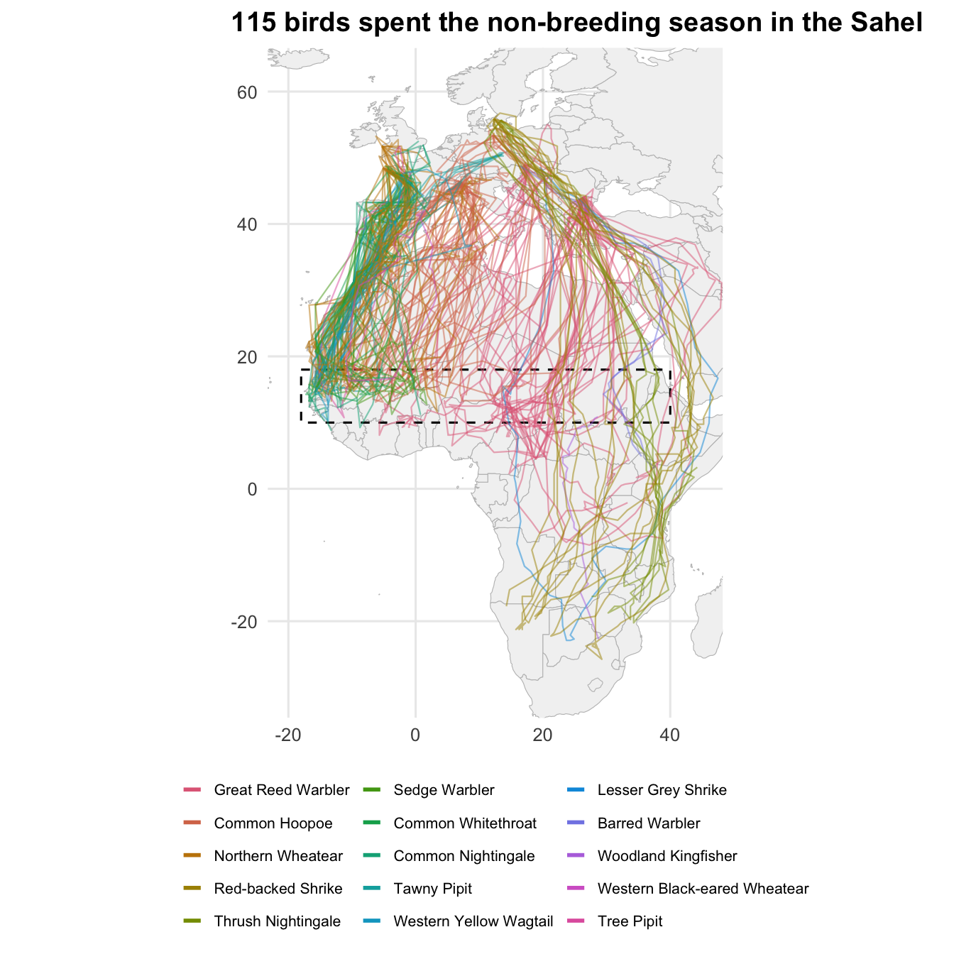

Migrants breeding from Iberia to Scandinavia and Eastern Europe share the Sahel: the Great Reed Warbler and the Common Hoopoe are the most tracked, but also wheatears, shrikes, nightingales and pipits.

The catalogue still lists every package of the Master. The datasets to cite with your results are those the selected birds come from:

sahel$datapackages |>
  semi_join(tags(sahel), by = "datapackage_id") |>
  transmute(citation = str_squish(bibliographicCitation), licenses) |>
  knitr::kable(col.names = c("Cite", "Licence"))

Cite	Licence
Nussbaumer R, Rime Y, Osinubi S (2025). “GeoLocator Data Package: South African Woodland Kingfisher.” doi:10.5281/zenodo.13829929 https://doi.org/10.5281/zenodo.13829929. https://zenodo.org/records/15259676.	Creative Commons Attribution 4.0 International (cc-by-4.0)
Nussbaumer R, Rime Y (2025). “Geolocator Data Package: Trajectories of Northern Wheatears breeding in Val Piora (Switzerland) and Val Troncea (Italy).” doi:10.5281/zenodo.14364135 https://doi.org/10.5281/zenodo.14364135. https://zenodo.org/records/14641780.	Creative Commons Attribution 4.0 International (cc-by-4.0)
Schaub M, Arlettaz R, Bauer S, van Wijk R, Liechti F, Bächler E, Capilla-Lasheras P, Nussbaumer R (2026). “GeoLocator Data Package: Swiss Hoopoes.” doi:10.5281/zenodo.14439689 https://doi.org/10.5281/zenodo.14439689. https://zenodo.org/records/23404056.	Creative Commons Attribution 4.0 International (cc-by-4.0)
Rime Y, Briedis M, Emmenegger T, Hahn S, Prochazka P, Kishkinev D, Bauer S, Nussbaumer R (2025). “GeoLocator Data Package: Great Reed Warbler tracks from three European populations.” doi:10.5281/zenodo.17084708 https://doi.org/10.5281/zenodo.17084708. https://zenodo.org/records/17084709.	Creative Commons Attribution 4.0 International (cc-by-4.0)
Adamik P, Wong J, Hahn S, Kristin A (2025). “GeoLocator Data Package: Lesser Grey Shrike in Slovakia.” doi:10.5281/zenodo.17257520 https://doi.org/10.5281/zenodo.17257520. https://zenodo.org/records/17257521.	Creative Commons Attribution 4.0 International (cc-by-4.0)
Wong J, Adamik P, Bažant M, Hahn S (2025). “GeoLocator Data Package: Barred Warblers from Czechia.” doi:10.5281/zenodo.17367319 https://doi.org/10.5281/zenodo.17367319. https://zenodo.org/records/17367320.	Creative Commons Attribution 4.0 International (cc-by-4.0)
Paul Doniol-Valcroze, Frédéric Jiguet, Sophie de Grissac, Pierrick Bocher, Yannig Coulomb, Fanny Rey, Rose Delacroix (2025). “GeoLocator Data Package: MIGRATLANE - Monitoring and studying birds in the North-East Atlantic Arc.” doi:10.5281/zenodo.17631330 https://doi.org/10.5281/zenodo.17631330. https://zenodo.org/records/17631331.	Creative Commons Attribution 4.0 International (cc-by-4.0)
Macías Torres P, Sjöberg S, Andersson A, Bäckman J, Thorup K, Tøttrup A, Alerstam T (2026). “Geolocator Data Package: Red-backed Shrike in Denmark.” doi:10.5281/zenodo.18311204 https://doi.org/10.5281/zenodo.18311204. https://zenodo.org/records/22294832.	Creative Commons Attribution 4.0 International (cc-by-4.0)
Macías-Torres P, Hedenström A (2026). “Geolocator Data Package: Thursh nightingale Luscinia Luscinia in South Sweden.” doi:10.5281/zenodo.18340650 https://doi.org/10.5281/zenodo.18340650. https://zenodo.org/records/18340651.	Creative Commons Attribution 4.0 International (cc-by-4.0)
Rime Y, Illa Llobet M (2026). “Geolocator Data Package: Western Black-eared Wheatear migration.” doi:10.5281/zenodo.18755137 https://doi.org/10.5281/zenodo.18755137. https://zenodo.org/records/18755138.	Creative Commons Attribution 4.0 International (cc-by-4.0)
Briedis M, Wong J, Beran V, Adamík P, Hahn S (2026). “GeoLocator Data Package: Tawny Pipits from Czechia.” doi:10.5281/zenodo.21376504 https://doi.org/10.5281/zenodo.21376504. https://zenodo.org/records/21376505.	Creative Commons Attribution 4.0 International (cc-by-4.0)
Zacmane E, Schmitz Ornés A, Kemper D, Bull K, Erselius M, Joisten F, Briedis M (2026). “GeoLocator Data Package: Eurasian Hoopoes from Germany.” doi:10.5281/zenodo.23211896 https://doi.org/10.5281/zenodo.23211896. https://zenodo.org/records/23211897.	Creative Commons Attribution 4.0 International (cc-by-4.0)

16.1.4 Back to the source package

The Master contains no raw measurements. To go back to the data of a bird, for instance to re-run its analysis with gldp_to_tag(), follow its datapackage_id and read the source package as described in Reuse a study:

doi <- tags(master) |>
  filter(tag_id == "16LP") |>
  pull(datapackage_id)

pkg <- read_zenodo(doi)

Build your own compilation

merge_gldp() combines any GeoLocator DPs into one, with the same datapackages catalogue as the Master. Use it to add packages that are not in the Master yet, such as embargoed data you have access to:

pkgs <- c("13829929", "16730669") |>
  purrr::map(read_zenodo) |>
  purrr::reduce(merge_gldp)

16.2 Migration across species

With all studies in one dataset, we can describe migration across species: how long birds stop, how long, when, how fast and how high they fly.

Projects differ in how many birds they tracked, for how long, and how often their tags sampled. A distribution over all flights would be dominated by the best-sampled projects. In the figures below, each bird weighs the same: its stops or flights get a weight of one over their number. Colours show the share of each species.

We keep birds with a trajectory of species with at least five of them, ordered by taxonomy.

birds <- tags(master) |>
  semi_join(paths(master), by = "tag_id") |>
  left_join(species, by = "scientific_name") |>
  filter(n() >= 5, .by = species) |>
  mutate(species = fct_reorder(species, Sequence)) |>
  select(tag_id, species)

Species colours

species_scale <- scale_fill_manual(
  values = setNames(hcl.colors(nlevels(birds$species), "Dark 3"), levels(birds$species)),
  name = NULL,
  guide = guide_legend(ncol = 4)
)

# Stacked density where each bird weighs the same (requires a `w` column)
plot_birds <- function(data, x, bw = "nrd0") {
  ggplot(data, aes({{ x }}, weight = w, fill = species)) +
    geom_density(aes(y = after_stat(wdensity)), position = "stack", bw = bw, colour = "white", linewidth = 0.1) +
    species_scale +
    labs(y = NULL) +
    theme(axis.text.y = element_blank(), panel.grid.major.y = element_blank())
}

That leaves 188 birds of 16 species.

16.2.1 How long do they stop?

A trajectory alternates stationary periods (staps) and flights (edges). We drop the first and last stationary period of each track, which are cut by the tag deployment and retrieval, and keep those of the most likely trajectory.

stays <- staps(master) |>
  inner_join(birds, by = "tag_id") |>
  semi_join(filter(paths(master), type == "most_likely"), by = c("tag_id", "stap_id")) |>
  filter(stap_id > min(stap_id), stap_id < max(stap_id), .by = tag_id) |>
  mutate(days = as.numeric(difftime(end, start, units = "days")), w = 1 / n(), .by = tag_id)

Code

plot_birds(stays, days, bw = 0.1) +
  geom_vline(xintercept = 14, linetype = "dashed") +
  scale_x_log10(
    breaks = c(0.25, 1, 7, 14, 60, 180),
    labels = c("6 h", "1 day", "1 week", "2 weeks", "2 months", "6 months")
  ) +
  labs(x = "Duration of stationary periods", title = "Most stops last a single day")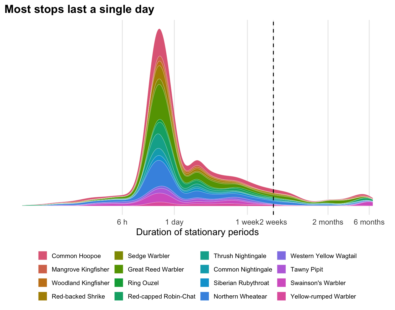

Durations span three orders of magnitude. Half of the stops last less than 20 hours: the bird lands at dawn and leaves the following night. Stays of several weeks or months (right of the dashed line, two weeks) mark the non-breeding grounds and major staging sites.

16.2.2 How long do they fly?

Each row of edges is a flight between two stationary periods. Flights with n > 1 span short stops that could not be located, so we keep single flights (n == 1). Flights with zero distance join two stationary periods in the same grid cell: they are local movements rather than migratory flights.

flights <- edges(master) |>
  filter(type == "most_likely", n == 1, distance > 0) |>
  inner_join(birds, by = "tag_id") |>
  mutate(w = 1 / n(), .by = tag_id)

Code

plot_birds(flights, flight_duration_h, bw = 0.07) +
  scale_x_log10(breaks = c(1, 2, 4, 8, 12, 24, 48)) +
  labs(x = "Flight duration (h)", title = "Most flights end before dawn")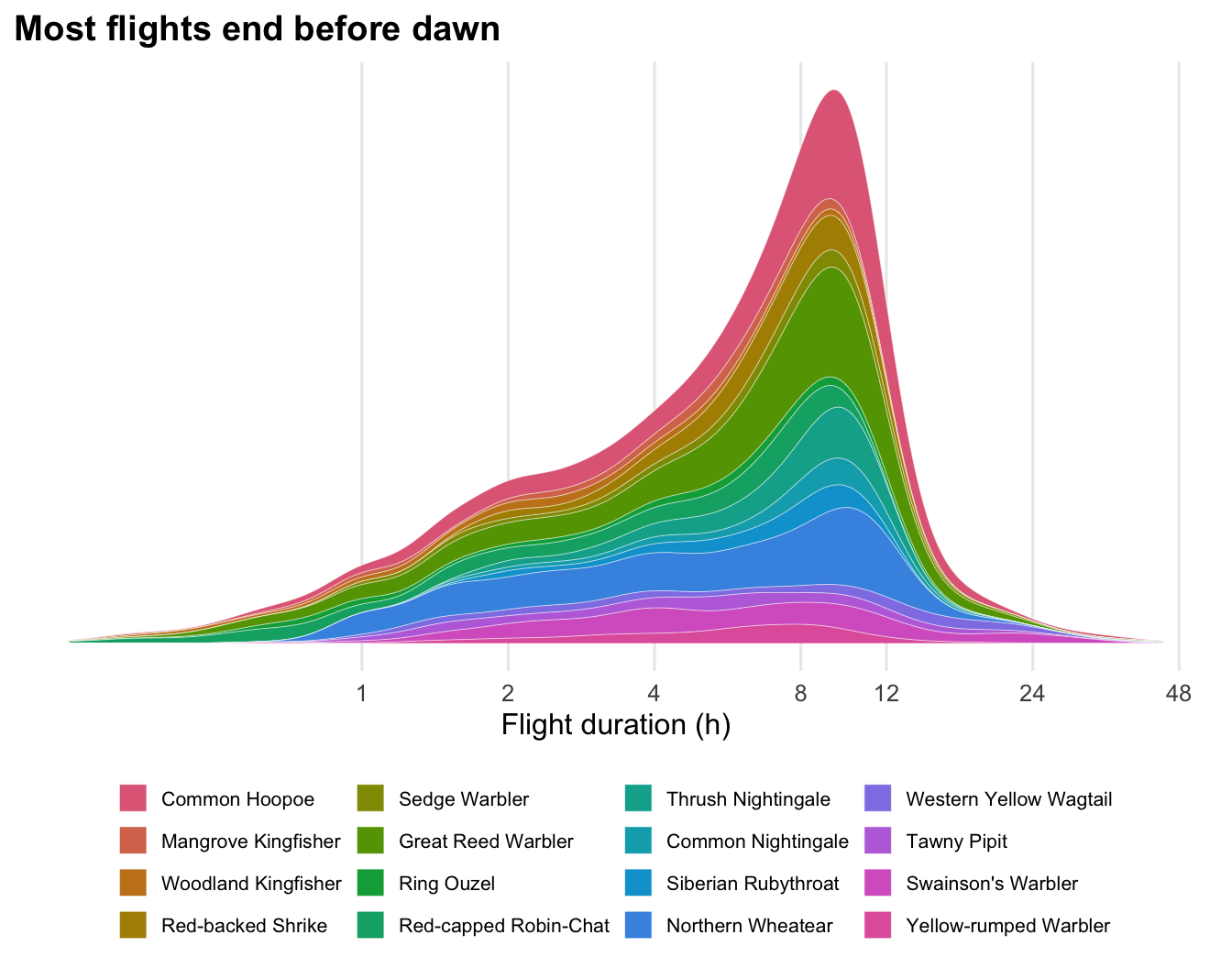

The median flight lasts 6.3 hours, and most stop at dawn, after 8 to 10 hours. Flights beyond 12 hours are non-stop crossings of the Sahara or the sea, continuing through the day.

16.2.3 When do they fly?

We place every 10 minutes of each flight on the local solar time, using the mean longitude of the flight (one hour per 15° of longitude), and weight them so that each bird’s flight time adds up to the same total.

airborne <- flights |>
  reframe(time = seq(start, end, by = "10 min"), .by = c(tag_id, species, stap_s, lon_s, lon_t)) |>
  mutate(
    solar_hour = (hour(time) + minute(time) / 60 + (lon_s + lon_t) / 2 / 15) %% 24,
    w = 1 / n(),
    .by = tag_id
  ) |>
  mutate(w = w / sum(w))

Code

# shift the hours to [12, 36) so that the night is in the middle
ggplot(airborne, aes((solar_hour - 12) %% 24 + 12, weight = w, fill = species)) +
  annotate("rect", xmin = 18, xmax = 30, ymin = -Inf, ymax = Inf, fill = "grey92") +
  geom_histogram(binwidth = 0.5, boundary = 0) +
  species_scale +
  scale_x_continuous(breaks = seq(12, 36, 3), labels = \(x) sprintf("%02d:00", x %% 24), expand = expansion(0)) +
  scale_y_continuous(labels = scales::percent) +
  labs(x = "Local solar time", y = "Share of flight time", title = "Migration happens at night") +
  theme(plot.margin = margin(5.5, 20, 5.5, 5.5))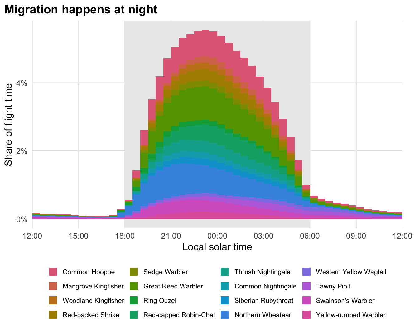

94% of the flight time falls between 18:00 and 06:00 solar time. What remains during the day are mostly the end of the longest flights.

Departure time is better measured from the actual sunset. The twilights table holds the sunrises and sunsets measured by each tag’s light sensor, at the bird’s own location. A rolling join with join_by(closest()) finds the last sunset before each departure:

sunsets <- twilights(master) |>
  filter(!rise, is.na(label) | label != "discard") |>
  select(tag_id, sunset = twilight)

departures <- flights |>
  inner_join(sunsets, by = join_by(tag_id, closest(start >= sunset))) |>
  # wrap to [-12, 12] h so that departures just before sunset are negative
  mutate(after_sunset = (as.numeric(difftime(start, sunset, units = "hours")) + 12) %% 24 - 12) |>
  mutate(w = 1 / n(), .by = tag_id)

Code

plot_birds(departures, after_sunset, bw = 0.15) +
  geom_vline(xintercept = 0, linetype = "dashed") +
  scale_x_continuous(breaks = seq(-12, 12, 2)) +
  coord_cartesian(xlim = c(-4, 10)) +
  labs(x = "Departure (hours after sunset)", title = "Birds take off soon after sunset")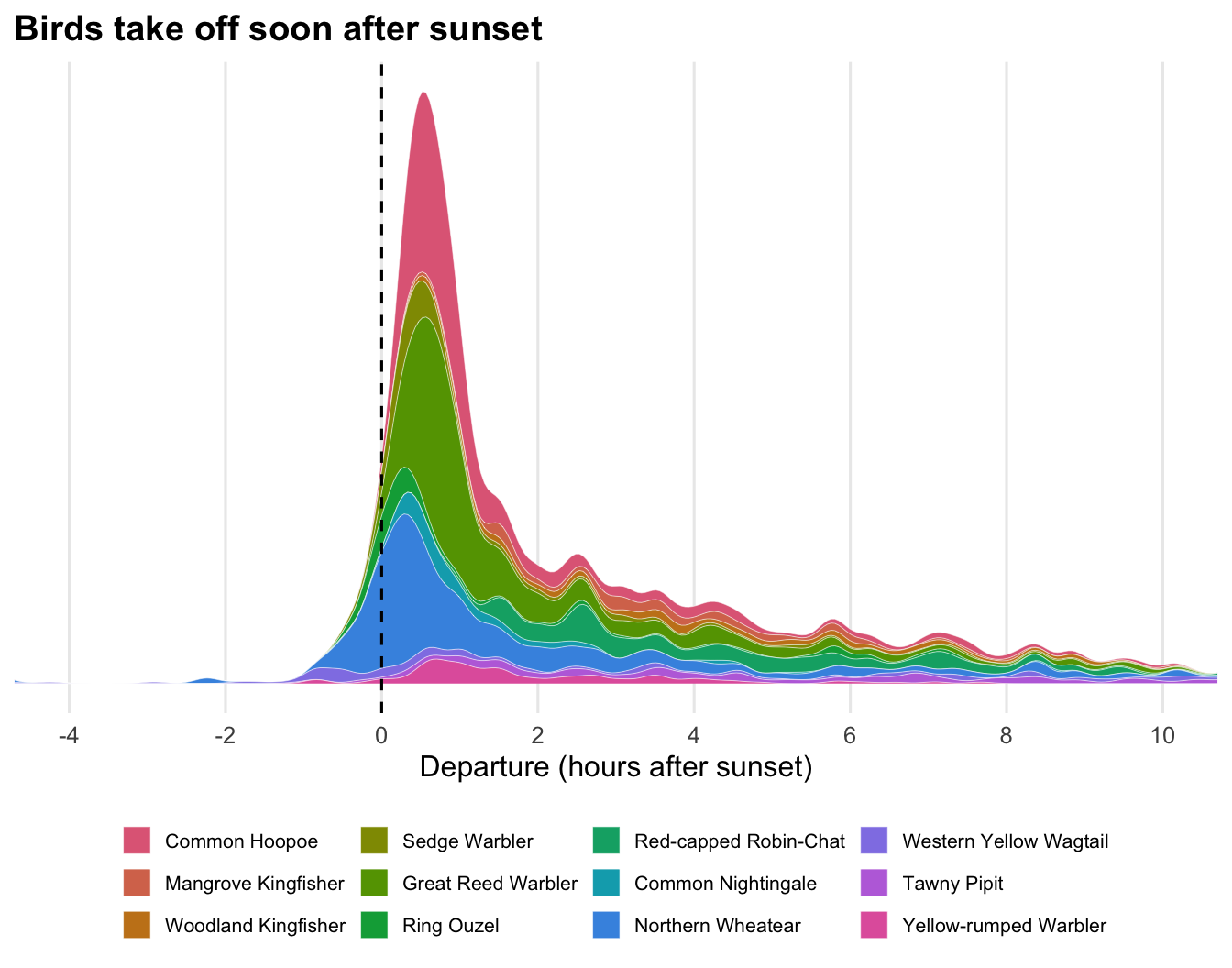

Half of the departures happen within 1.1 hours of sunset. Species without twilights in the Master are missing from this figure.

16.2.4 How fast do they fly?

edges store the bird’s ground velocity (gs_u, gs_v) and the ERA5 wind it experienced (ws_u, ws_v), as eastward and northward components in km/h. The difference is the airspeed, the speed of the bird relative to the air, and the wind support is the wind component along the direction of travel. Wind is only available for trajectories computed with a wind model.

flights <- flights |>
  mutate(
    ground_speed = sqrt(gs_u^2 + gs_v^2),
    air_speed = sqrt((gs_u - ws_u)^2 + (gs_v - ws_v)^2),
    wind_support = (ws_u * gs_u + ws_v * gs_v) / ground_speed
  )

fit <- lm(ground_speed ~ wind_support, data = flights)

Code

flights |>
  filter(!is.na(wind_support)) |>
  ggplot(aes(wind_support, ground_speed)) +
  geom_point(aes(colour = species), alpha = 0.25, size = 0.6) +
  geom_abline(intercept = coef(fit)[1], slope = coef(fit)[2], linewidth = 0.8) +
  geom_vline(xintercept = 0, linetype = "dashed") +
  scale_colour_manual(
    values = setNames(hcl.colors(nlevels(birds$species), "Dark 3"), levels(birds$species)),
    name = NULL, guide = guide_legend(ncol = 4, override.aes = list(alpha = 1, size = 2))
  ) +
  coord_cartesian(xlim = c(-60, 80), ylim = c(0, 150)) +
  labs(x = "Wind support (km/h)", y = "Ground speed (km/h)", title = "Tailwinds make birds faster")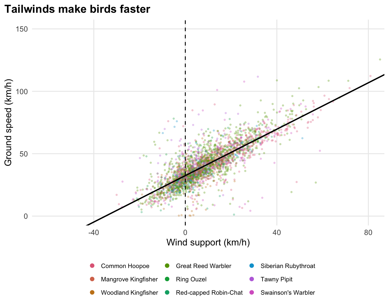

Birds fly at a median airspeed of 33 km/h. 74% of the flights had a tailwind, and each km/h of wind support adds 0.93 km/h to the ground speed. Birds barely lower their airspeed when the wind helps them: they simply travel faster.

16.2.5 How high do they fly?

The pressure sensor that locates a bird on the ground also gives its altitude in flight. pressurepaths follow the most likely trajectory at the tag’s sampling interval. Flight samples are the rows with a fractional stap_id, between stap_s and stap_s + 1. We drop samples labelled discard and summarise each flight by its median and maximum altitude.

altitude <- pressurepaths(master) |>
  filter(type == "most_likely", stap_id %% 1 != 0, !is.na(altitude), is.na(label) | label != "discard") |>
  inner_join(birds, by = "tag_id") |>
  mutate(stap_s = floor(stap_id)) |>
  summarise(max_altitude = max(altitude), altitude = median(altitude), .by = c(species, tag_id, stap_s)) |>
  mutate(w = 1 / n(), .by = tag_id)

Code

plot_birds(altitude, altitude) +
  scale_x_continuous(labels = scales::label_comma(suffix = " m")) +
  coord_cartesian(xlim = c(0, 5000)) +
  labs(x = "Median altitude of each flight (above sea level)", title = "Most flights cruise between a few hundred and 2,000 m")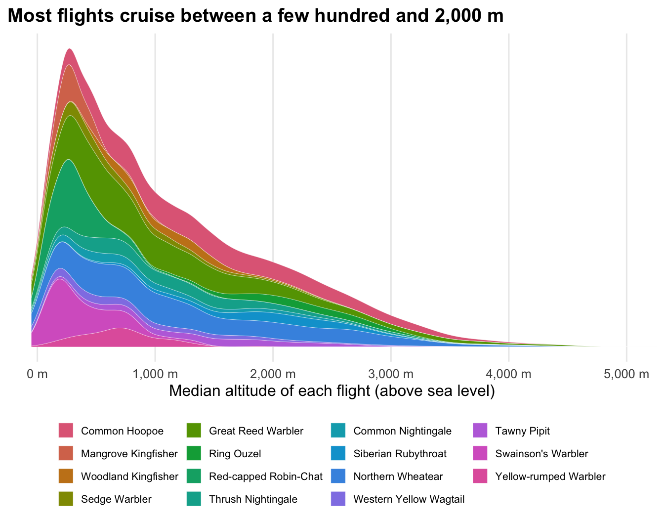

The median flight cruises at 930 m, and the highest point of half of the flights is above 1,680 m. Altitudes are above sea level, not above ground: a bird crossing a high plateau flies high without climbing much.

16.2.6 Species profiles

To compare species, we summarise each bird first, then take the median across the birds of each species.

per_bird <- list(
  stays |>
    summarise(stopover_d = median(days[days < 14]), .by = c(species, tag_id)),
  flights |>
    summarise(
      flight_h = median(flight_duration_h),
      longest_h = max(flight_duration_h),
      air_speed = median(air_speed, na.rm = TRUE),
      .by = c(species, tag_id)
    ),
  departures |>
    summarise(after_sunset_h = median(after_sunset), .by = c(species, tag_id)),
  altitude |>
    summarise(altitude = median(altitude), max_altitude = max(max_altitude), .by = c(species, tag_id))
) |>
  reduce(full_join, by = c("species", "tag_id"))

Code

per_bird |>
  summarise(birds = n(), across(-tag_id, \(x) median(x, na.rm = TRUE)), .by = species) |>
  arrange(species) |>
  knitr::kable(
    digits = 1,
    col.names = c(
      "Species", "Birds", "Stopover (d)", "Flight (h)", "Longest flight (h)",
      "Airspeed (km/h)", "Departure after sunset (h)", "Altitude (m)", "Max altitude (m)"
    )
  )

Species	Birds	Stopover (d)	Flight (h)	Longest flight (h)	Airspeed (km/h)	Departure after sunset (h)	Altitude (m)	Max altitude (m)
Common Hoopoe	28	0.7	7.6	15.5	32.5	0.8	1352.6	4414.5
Mangrove Kingfisher	5	0.8	4.9	9.5	32.9	3.4	266.8	1126.1
Woodland Kingfisher	5	0.9	3.2	11.0	34.5	4.0	1135.8	2688.2
Red-backed Shrike	10	0.8	7.0	14.0
Sedge Warbler	6	0.8	6.7	18.2		0.6	519.8	4554.5
Great Reed Warbler	32	0.7	7.5	17.3	32.6	0.9	789.1	5975.3
Ring Ouzel	5	1.0	2.9	12.2	35.6	0.5	2149.7	4098.9
Red-capped Robin-Chat	13	0.9	3.7	8.8	31.0	3.8	250.9	1436.0
Thrush Nightingale	11	0.7	8.0	12.0			1025.0	5026.7
Common Nightingale	6	0.7	8.2	16.8		0.8	675.8	4291.9
Siberian Rubythroat	6	1.5	7.0	10.0	30.7		1984.6	3814.6
Northern Wheatear	29	0.7	5.3	13.0		0.5	1108.4	4070.2
Western Yellow Wagtail	6	0.9	7.0	23.5		2.0	599.5	3956.4
Tawny Pipit	7	0.9	4.7	20.2	36.4	4.8	1489.3	3236.8
Swainson’s Warbler	13	0.8	5.0	21.0	33.2		251.7	1674.4
Yellow-rumped Warbler	6	1.8	6.1	12.2		1.3	692.5	2097.1

Empty cells are species whose projects have no wind model, no twilights or no pressurepaths in the Master.

16.3 Cite the data

Cite the Master release you used and the source packages that contributed the birds of your analysis (see Select birds by what they did). Most packages are under CC BY 4.0. If your results rely on a few projects, contact their authors: they know their data best.